Zero-Event Samples
Two fictional loan samples show no missed payments. Their matching percentages conceal different amounts of evidence under the same assumptions.
Estimated reading time: 5 minutes
Two fictional loan samples show no missed payments. Their matching percentages conceal different amounts of evidence under the same assumptions.
State the experiment before reading the percentage
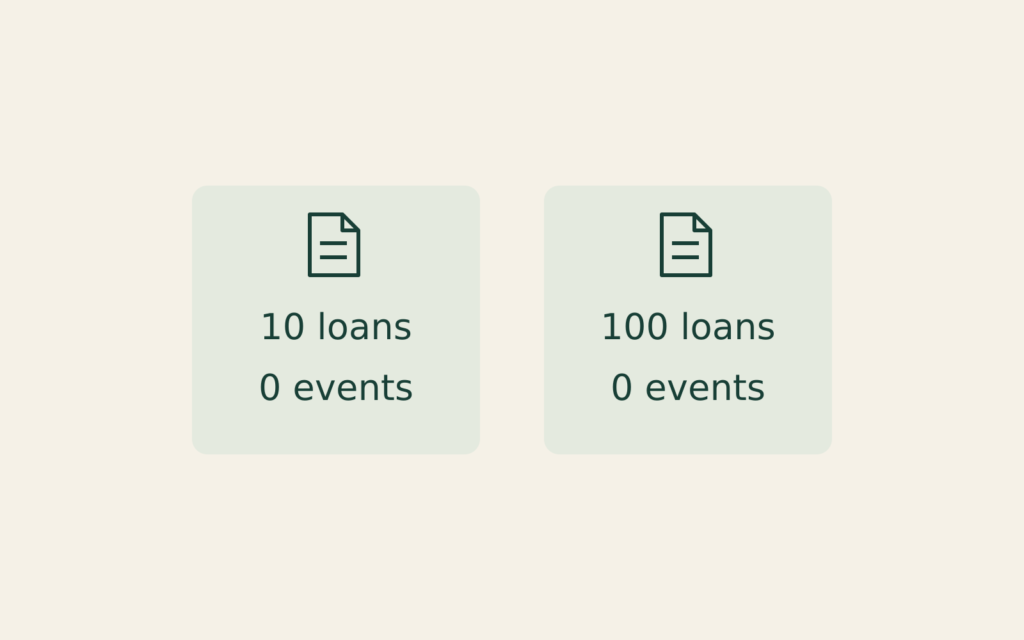
Imagine two independently assembled samples. Their sizes are fixed before outcomes are observed: one contains 10 loans; the other contains 100. Every loan has been observed for its entire first year. For this exercise, an event means at least one scheduled payment was missed during that year. Both samples contain zero events. Their observed event fractions are therefore 0/10 and 0/100, both 0%.
Now stipulate a deliberately simplified model: every loan has the same underlying event probability, called p, and learning any other outcomes does not change a loan’s probability. These are assumptions for the arithmetic, not findings about actual borrowers. No lender, credit score or real portfolio is represented. A loan contributes one outcome, not twelve independent observations merely because it has twelve payment dates.
Ask how surprising zero would be
Test a hypothetical event probability of 5%. Under that assumption, each loan has a 95% chance of no event. For two independent loans, the chance that both have no event is 0.95 × 0.95. For ten, multiply ten copies of 0.95. For one hundred, multiply one hundred copies.
| Fictional sample | Observed events | Calculation under p = 5% | Chance of zero |
|---|---|---|---|
| 10 loans | 0 | 0.95^10 | 59.87% |
| 100 loans | 0 | 0.95^100 | 0.59% |
Zero is quite unsurprising in the ten-loan experiment even when the assumed event probability is 5%. It is much less common in the hundred-loan experiment under exactly that same probability. Matching observed percentages therefore do not make the evidence interchangeable.
The last column is not the probability that p equals 5%. We supplied p first and calculated the chance of an observation. Reversing that conditional question requires more than reading the table backward. Nor does the larger sample prove that the next borrower will pay: the calculation concerns the joint outcome of a stipulated experiment.
Turn the question around algebraically
Choose a separate threshold: how large could p be before an all-zero result has only a 5% chance? This second 5% is a chosen tail threshold, not the event probability tested above. They happen to share a number, but perform different jobs.
For n independent outcomes, the zero-event probability is (1 − p)^n. Set that expression equal to 0.05. Taking the nth root gives 1 − p = 0.05^(1/n), so the boundary is p = 1 − 0.05^(1/n).
| Sample size n | Boundary p | Substitution with additional digits |
|---|---|---|
| 10 | 25.89% | (1 − 0.2588655509)^10 ≈ 0.05 |
| 100 | 2.95% | (1 − 0.0295130496)^100 ≈ 0.05 |
For probabilities above the relevant boundary, getting zero becomes even less likely: subtracting a larger p leaves a smaller number to multiply. Below the boundary, zero is more likely. This establishes a transparent comparison without pretending that the observed 0% is the only possible underlying probability.
Do not turn a chosen boundary into a guarantee
The two boundaries answer the same chosen question with different sample sizes. Neither is a maximum possible future realized event fraction. A future group can experience an unusual outcome. Neither states that there is a 95% probability that this particular unknown p lies below the displayed number.
NIST explains confidence levels through repeated sampling and the proportion of resulting intervals that contain the population parameter. It also distinguishes one-sided bounds from two-sided intervals. Here the displayed calculation is explicitly a chosen zero-event tail boundary, rather than an invitation to apply a confidence-interval label to any lender’s statistics.
Find the integer boundary
The same arithmetic identifies an integer boundary. Keeping the hypothetical event probability at 5%, how many independent outcomes would make zero occur less than 5% of the time? Solving 0.95^n = 0.05 gives n ≈ 58.404. Rounding down would be wrong: 0.95^58 is about 5.10%, still above the chosen threshold. At 59 outcomes, 0.95^59 is about 4.85%, below it. This does not promise that collecting 59 observations will produce zero events. It specifies what an all-zero result would mean under the assumed model, if that result occurred.
Duplicating records cannot manufacture evidence
Suppose someone takes the ten original loan records and copies each row ten times. The spreadsheet now has 100 rows and still shows zero events. But it has only ten distinct loan outcomes. Each repeated row must match its original; those copies are not independent outcomes. Under our original experiment, the chance of all-zero records remains 0.95^10, not 0.95^100. Counting rows instead of distinct observations would produce the smaller boundary without obtaining the additional evidence that justified it.
Keep the model separate from a lending conclusion
NIST’s binomial description concerns two mutually exclusive outcomes and a probability fixed across trials. Actual loan groups need not fit that model. This exercise supplies no evidence that different borrowers share one probability or that their outcomes are independent.
The 2021 ASA President’s Task Force statement emphasizes study design, measurement, model choice and transparent reporting. It distinguishes statistical assessments from practical importance. Our calculation can expose an unsupported inference from “zero,” but cannot choose a lender, set an affordable payment or establish anyone’s personal repayment probability.
Deferred Compensation
A deferred-compensation statement and payroll form can describe different rights and events.
Loan Horizons
A smaller cumulative missed-payment count can reflect a shorter observation window. This fictional record exercise compares equal payment ages instead.
Rate Transmission
A rate announcement, a market yield and a contract reset describe different links between monetary policy and borrowing costs.