Household Debt Service Ratio: Check the Method Before Joining Two Series
Use a fictional two-period table to separate a within-method change from a mixed-method gap, then test a constant-adjustment shortcut.
Estimated reading time: 5 minutes
A chart can show an apparent jump because its author joined numbers calculated differently. Before describing a change in household debt burdens, check whether the observations belong to the same measurement method.
This guide separates a documented Federal Reserve change from a fictional spreadsheet exercise. The exercise shows how to repair a comparison, not how to estimate any missing U.S. figure.
What changed in the Federal Reserve series?
The household debt service ratio, or DSR, compares total required household debt payments with disposable personal income. Mortgage and consumer components add to the total. The Federal Reserve’s current method uses scheduled payments reported in credit bureau records; its previous method estimated payments from balances, interest rates and remaining terms. Current-method quarterly history begins in 2005; previous-method history runs from 1980 through 2024. See the Fed’s methodology overview.
The previous release page identifies the transition as beginning with the 2024 second-quarter DSR publication. A historical date alone therefore doesn’t identify which method a downloaded observation uses.
Daniel Ringo’s September 2024 FEDS Note explains an important coverage difference: the credit-bureau measure includes mortgage escrow amounts bundled into reported payments, whereas the old measure targeted principal and interest. The note also describes differences in the series’ movements, not just their levels. It doesn’t provide a universal constant to add to every old observation.
Use a two-method, two-period worksheet
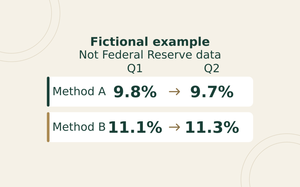
Imagine two invented methods, A and B, applied to the same two fictional quarters. Each cell below is a stipulated percentage, not a Federal Reserve observation, reconstruction or forecast. No actual debt payments, income totals or escrow amounts are inferred from these numbers.
| Period | Method A | Method B |
|---|---|---|
| Quarter 1 | 9.8% | 11.1% |
| Quarter 2 | 9.7% | 11.3% |
Suppose a spreadsheet retains only A’s Quarter 1 value and B’s Quarter 2 value. Subtracting 9.8% from 11.3% gives an apparent rise of 1.5 percentage points. The subtraction is correct. Calling it the change measured by either method isn’t.
Under A, the within-method movement is 9.7% minus 9.8%: a fall of 0.1 percentage point. Under B, it’s 11.3% minus 11.1%: a rise of 0.2 percentage point. The diagonal comparison has mixed a period change with a method difference.
Reconcile the apparent jump in two ways
Start at A’s Quarter 1 value of 9.8%. Move across the first row to B’s 11.1%, a difference of 1.3 percentage points. Then move down B’s column to 11.3%, another 0.2 point. Together, 1.3 + 0.2 = 1.5.
Alternatively, move down A’s column first: 9.8% to 9.7%, or minus 0.1 point. Then cross the second row to B’s 11.3%, a 1.6-point difference. Again, minus 0.1 + 1.6 = 1.5.
Both routes reconcile the same endpoints. They don’t prove which method is more accurate, why either series changed, or how much of a real-world change came from any particular cause. Their purpose is to expose the missing comparisons hidden by the diagonal.
Why one adjustment doesn’t fix the exercise
The first-quarter gap between B and A is 1.3 points. Adding that constant to A’s second-quarter 9.7% produces 11.0%, not the stipulated B value of 11.3%. The proposed shortcut misses by 0.3 point because the second-quarter gap is 1.6 points.
Using the second-quarter gap to adjust the first quarter fails in the other direction: 9.8% + 1.6 points = 11.4%, rather than 11.1%. One matching quarter cannot establish that the relationship remains constant elsewhere.
If B’s first-quarter observation were missing, this exercise wouldn’t let you calculate it from the other three cells without an additional assumption. Mark the cell unavailable. Don’t quietly replace it with A’s value and present the result as a continuous B history.
Repair a saved chart before interpreting it
Keep the original download and make a working copy. Beside each observation, record the period, series name, method, units and download date. Identify where a copied table or chart switches sources. A neatly connected line isn’t evidence that these labels match.
For periods where the desired method is available, rebuild the comparison using that method on both dates. If the requested span can’t be covered consistently, shorten the span or show separate, clearly labeled series. Don’t hide a missing observation with a line that implies an observed value.
Write the chart’s conclusion only after this check. For the invented table, an accurate statement is: “Method B rises 0.2 percentage point between the two quarters; the mixed-method endpoints differ by 1.5 points.” It would be inaccurate to describe the entire 1.5-point gap as the change within B.
Finally, keep this research exercise separate from a borrowing decision. It supplies no household payment schedule, loan approval threshold or personal affordability result. For an individual calculation, use the actual included obligations and income definition, as explained in our debt-to-income input guide.
General U.S. financial education, not individualized advice. Sources checked October 29, 2026. All table values and worked comparisons are fictional.
Deferred Compensation
A deferred-compensation statement and payroll form can describe different rights and events.
Loan Horizons
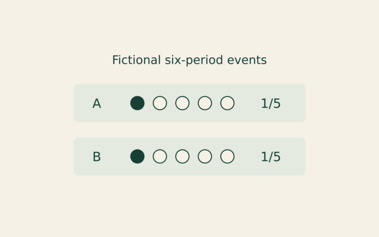
A smaller cumulative missed-payment count can reflect a shorter observation window. This fictional record exercise compares equal payment ages instead.
Rate Transmission
A rate announcement, a market yield and a contract reset describe different links between monetary policy and borrowing costs.