Alert Accuracy
A fictional payment-screening rule achieves 99% accuracy in two datasets. Yet the composition of its alerts differs substantially between them.
Estimated reading time: 5 minutes
A fictional payment-screening rule achieves 99% accuracy in two datasets. Yet the composition of its alerts differs substantially between them.
Hold the rule fixed, change the mix
Construct two files containing 10,000 payment records each. Every record has a stipulated correct label: a specified payment error is either present or absent. These are invented validation records, not transactions from a bank or estimates of any actual system’s performance.
In both files, the rule flags exactly 99% of error-present records and exactly 1% of error-absent records. The first percentage measures successful detection within the error-present group. The second measures false alarms within the error-absent group. We change neither percentage between files; only the prevalence of the specified error changes.
Build both complete count tables
File A contains 100 error-present records and 9,900 error-absent records. Flagging 99% of the first group produces 99 true alerts and one missed error. Flagging 1% of the second produces 99 false alerts, leaving 9,801 correctly unflagged records.
File B contains 1,000 error-present records and 9,000 error-absent records. The identical percentages produce 990 true alerts, ten missed errors, 90 false alerts and 8,910 correctly unflagged records.
| Outcome | File A | File B |
|---|---|---|
| True alert | 99 | 990 |
| Missed error | 1 | 10 |
| False alert | 99 | 90 |
| Correctly unflagged | 9,801 | 8,910 |
| Total records | 10,000 | 10,000 |
The four outcomes exhaust each file. A record cannot simultaneously be a true alert and a false alert: its stipulated label determines which description applies. The table therefore provides a check on both the arithmetic and the denominator used next.
Check what the matching accuracy conceals
Accuracy counts both kinds of correct classification. File A has 99 + 9,801 = 9,900 correct results. File B has 990 + 8,910 = 9,900. Both therefore reach 99% accuracy, and both contain exactly 100 mistakes.
But their mistakes differ. File A misses one error and generates 99 false alerts; File B misses ten errors and generates 90 false alerts. The shared total does not preserve the mix of mistakes. Nor does it preserve the number of alerts: A has 198, while B has 1,080.
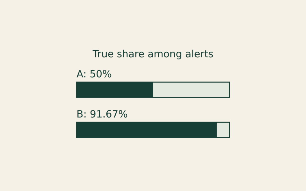
Among A’s alerts, 99/198 = 50% are true alerts. Among B’s, 990/1,080 ≈ 91.67% are true alerts. The rule’s two stipulated operating percentages stayed fixed throughout. Changing the underlying mix alone changed what a flagged group contains.
Keep the two false-alarm denominators separate
In File A, 99 false alerts divided by 9,900 error-absent records gives the stipulated 1% false-alarm rate. Those same 99 false alerts divided by all 198 alerts give a 50% false-alert share. These are not conflicting calculations; they answer different questions.
For File B, the corresponding calculations are 90/9,000 = 1% and 90/1,080 ≈ 8.33%. Thus “1% of error-absent records were flagged” does not mean “only 1% of flags were false.” The changed prevalence affects the second fraction even while the first stays fixed.
Check the unflagged records too
File A leaves 9,802 records unflagged: 9,801 are correctly unflagged and one contains a missed error. Its error share among unflagged records is approximately 0.0102%. File B leaves 8,920 unflagged, including ten missed errors, for approximately 0.1121%. The stipulated 1% miss rate uses error-present records as its denominator; neither of these unflagged-group percentages uses that denominator. Changing the mix affects both sides of the classification table.
Prove where the balance changes
Let p represent the fraction of records containing the specified error. Per record, the construction supplies 0.99p true alerts and 0.01(1 − p) false alerts. The true share among alerts is therefore:
0.99p ÷ [0.99p + 0.01(1 − p)].
True alerts outnumber false alerts exactly when 0.99p > 0.01(1 − p). Rearranging gives p > 0.01. At 1% prevalence, the two alert types tie, as in File A. Above that prevalence, true alerts form the majority under this stipulated rule.
For a true-alert share of at least 90%, solve 0.99p ≥ 0.90[0.98p + 0.01]. This becomes 0.108p ≥ 0.009, or p ≥ 1/12, approximately 8.33%. File B’s 10% prevalence satisfies that condition. This is a boundary for the dataset’s composition, not a recommendation to change a model’s flagging threshold.
The constant accuracy also has a precise explanation: 0.99p + 0.99(1 − p) = 0.99. Both within-class correct-classification rates happen to be 99%. Accuracy would not generally remain constant as prevalence changed if those two percentages differed.
Use the definitions without inventing a verdict
Google’s classification guide distinguishes accuracy, recall, false-positive rate and precision by their denominators. Precision concerns the positive classifications that are actually positive; it is not another name for overall accuracy. The guide also explains that meaningful evaluation depends on the task and the costs of different mistakes.
Here the labels and percentages are assumptions, not measured facts about an institution. The exercise does not establish that a particular payment is erroneous, that an alert warrants refusing credit, or that one real system is preferable. Its narrower result is demonstrable: the same accuracy headline and conditional rates can accompany different alert compositions when the underlying mix changes.
Deferred Compensation
A deferred-compensation statement and payroll form can describe different rights and events.
Loan Horizons
A smaller cumulative missed-payment count can reflect a shorter observation window. This fictional record exercise compares equal payment ages instead.
Rate Transmission
A rate announcement, a market yield and a contract reset describe different links between monetary policy and borrowing costs.